Visualizing and Refining Terrain Survey

Introduction
The objective for this week's exercise was to import the spatial data collected from our terrain survey last week and project it into a model in ArcGIS. In order to create a three dimensional model we used various methods of interpolation including:

• IDW
• Natural Neighbor
• Kriging
• Spline
• TIN

After creating and analyzing the models we decided to resample our area using different sampling protocols in order to create the most spatially accurate model as possible. Because of rain distorting our survey area, it was rebuilt on top of the first, maintaining the same features in the same location (Figure 1).Our group decided to resurvey the entire terrain collecting more XYZ coordinate points at the areas that resulted in accurate modeling such as on slopes and within depressions. Using the new coordinates we reran the interpolation methods to produce a more accurate model.

The goals of this lab were to determine the most efficient surveying techniques to create accurate models. We were to learn about interpolation methods, how to implement them, and the advantages and disadvantages of using each kind of method. We also learned about improving our surveying techniques; balancing collection efforts and data efficiency. This lab taught us very useful survey skills we can implement in a variety of future situations.

Figure 1. Landscape features from left to right: Depression, Ridge, Valley, Hill, Plain

Methods
After we collected the initial survey XYZ data in an Excel spreadsheet and formatted it, the data was imported into ArcGIS and saved in a feature class within a geodatabase created for this lab activity.
Various interpolation methods were performed with the data. ArcGIS Help defines interpolation as predicting values for cells in a raster from a limited number of sample data points. Interpolation is a way to convert individual point values into a continuous raster feature by 'filling in the blanks' between points.  Many different interpolation methods are utilized to achieve different results as required by the surveyor (Figure 2).The rasters and TIN that were created using the methods discussed below were viewed in ArcScene in order to view the models in 3D to better analyze the effectiveness of each.

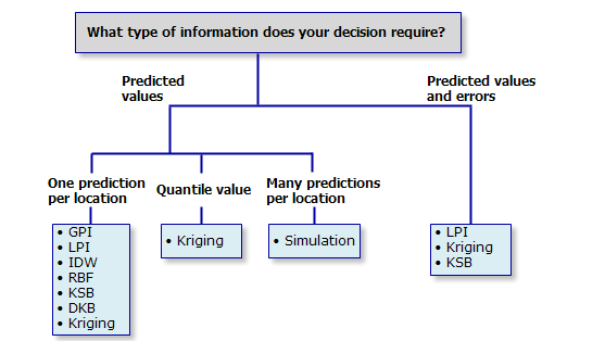Figure 2. Different interpolation methods may be used based on the requirements of the data.

The first method of interpolation used was IDW, or Inverse Distance Weighted technique. This method averages cell values by averaging the values of the points near each cell. The closer a point is to the cell , the more weight it is assigned in the averaging process. Because areas are less accurate the farther away they are from the points, it can cause problems on areas with a steep slope change such as on ridges or valleys.

Figure 3. 3D model of the survey area using the IDW interpolation method. The bumps and pock marks are the result of areas farther away from the coordinate points being weighted less and decreasing the influence of the raster cell.

The second interpolation method that was utilized was the Natural Neighbor method. An advantage of this method is that it doesn't make many assumptions about the data and only takes into consideration the nearest points to determine cell value. Because of this, the Natural Neighbor method is best utilized on projects that require fine detail. This method will not predict trends. This method employs "area stealing" meaning that it uses the nearest coordinate points and weigh them based on their proportionate areas. A disadvantage is that if a cell center falls outside of the convex cell as defined by the input points, those cells will be assigned a value of NoData.

Figure 4. 3D model of the survey area using the Natural Neighbor interpolation method. This method uses "area stealing" based on nearby coordinate points. This results in a smooth surface relative to the IDW method.

The next interpolation method used was Kriging. Kriging creates an estimated surface and utilizes trend to create a raster surface. A disadvantage of Kriging is that it can be processer-intensive if many points are processed. Kriging assumes the presence of a structural component and assumes that local trends vary among locations.

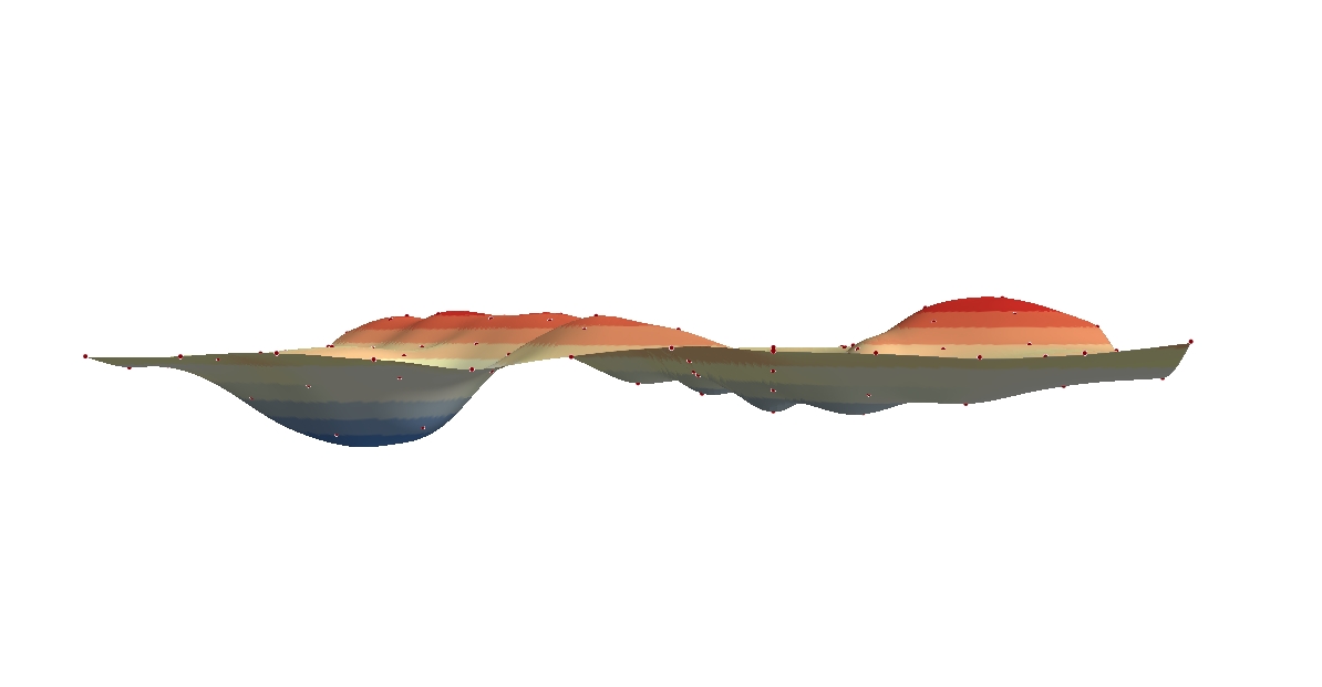
Figure 5. 3D model of the survey using the Kriging interpolation method. Because Kriging takes into account the overall spatial arrangement, it can predict the terrain features using trends.

The fourth interpolation model we tested was Spline. The Spline method used a mathematical function to reduce surface curvature which effectively smoothed the raster to fit perfectly through each coordinate point. Although aesthetically pleasing, some surface features may be ignored if they don't occur directly on the collected coordinate points. Accuracy may be increased by increasing the number of XYZ coordinate points collected.

Figure 6. 3D model of the surveyed terrain using the Spline interpolation method. This method allows for the raster to smoothly fit through each collected coordinate point at the expense of losing the undocumented terrain variation.

The final interpolation method we utilized was TIN, or Triangle Irregular Network. TIN is often used to represent surface morphology digitally. TIN utilizes contiguous triangular facets to create 3D images which is different from the other interpolation methods. TIN preserves the integrity of nodes and edges and is often utilized to accurately model ridges and areas with steeply changing values. A disadvantage is that although it produces an accurate model using the input points, it lacks realism and creates many sharp lines that do not exist in nature.

Figure 7. 3D model of the terrain created by making a TIN. Unlike the rasters, this model uses triangles and maintains the data integrity of all of the input coordinate points.

Initially, our group decided that Spline best represented our surveyed data but we believed that we could improve our surveying techniques and create an even more accurate model. In order to better represent the features in our terrain we altered our coordinate grid and collected some points at a 5cm scale around the features which had a significant terrain change such as the ridge, depression, valley, and hill (Figure 8). The plain feature's data collection was not altered as there was little change in the terrain of that feature.

Figure 8. The collected XYZ coordinate system of the initial survey as compared to the XYZ coordinate system collected in the second survey.

In order to take methods using a 5cm scale at some areas, we marked measurements on masking tape on the frame of the survey box in both 5cm and 10 cm increments (Figure 9).

Figure 9. Marking masking tape on the top of the frame with 5cm and 10cm increments.

In order to make data collection more time efficient and accurate, for the second survey instead of using string we laid a expandable measuring tape across the frame which allowed us to take measurements with another measuring stick without having to move strings for each new point (Figure 10).

Figure 10. A measuring stick was laid across the frame in lieu of string in order to more efficiently and accurately record XYZ coordinate points.

In response to concerns raised during the initial survey, we dug out the outline of the frame so that points with no height features would be flush with 'sea level.' The frame was leveled with a digital level from our smartphones. Because we had to rebuild our feature's surfaces which had been altered from the rain, it was not crucial to match up our initial grid to the subsequent one. In total we collected 218 points as compared to 132 points in the first survey. We hoped that after importing our data into ArcGIS and rerunning the interpolation methods, we would find that our rasters were more representative of the real life terrain. After running the Spline interpolation, we determined that the new model including the more detailed method gave us a more spatially accurate raster (Figure 11).


Figure 11. Model with more XYZ coordinate points than the first survey and a Spline interpolation is a more accurate representation of our terrain.

Discussion
The main issue we faced when tasked with creating a second survey was improving how the data was collected so that the terrain features would be more representative of our physical terrain. We solved this issue by collecting points in between the original coordinate points by measuring 5cm intervals at features that had a significant change in topology that we wanted to account for in our models. The improvements were observed using each of the interpolation methods are shown below.

 

Figure 12, Model of initial survey using the Spline interpolation method. Some terrain features, especially elevation gradients on slopes have been 'averaged out' resulting in an aesthetically pleasing, but slightly spatially inaccurate model.

 

Figure 13. Model of second survey using the Spline interpolation method. By collecting additional points where there were elevation gradients, the features that were smoothed out in the initial survey are now accounted for in the second survey model.

 It is important to realize that our surveys were not perfect replicates of each other due to the need to rebuild the features. However, it is clear that the second method using more XYZ in areas that had gradient changes greatly improved the accuracy of our model.

 Some challenges and sources of error that we ran into were the same as those experienced in the initial survey. Because of the fragile nature of sand based structures, a very delicate hand was needed in order to obtain an accurate measurement while maintaining the integrity of the terrain. Obtaining measurements from surface level was especially hard in the middle of the frame because we could not lean on the frame lest we disturb the leveling nor could we hold ourselves up in the terrain without altering the geography. Abdominal training may have lessened our challenge.

An issue unique to the second survey was the issue of time. The second survey was recorded in the morning, and we finished just in time for me to reach my next class in time. Due to the time crunch we may have been less careful than we would have been otherwise.

A challenge that we solved during the second survey was remembering to dig out where the frame sat in the sand so that areas with no height were at or within a positive sea level value. Light was better in the morning and resulted in more spatially representative photographs.

Conclusion
Although during the second survey we solved many of our issues, I believe that there is still room for improvement, as there is in any project. Packing the sand or keeping it sufficiently wet may help for maintaining terrain integrity and even more XYZ coordinate points may improve our rasters. Although we had to completely resurvey our area, I feel that we improved not only our methods but also the accuracy of our raster. In doing so, we accomplished the main objective of this exercise which was to improve on our survey methods and ability to use interpolation methods to accurately represent a surveyed terrain.

References: ArcGIS Help Online