Exercise 1: Metadata Sandbox Terrain Survey

Collectors:
Katie Lueth
Peter Sawall
Zach Nemeth

Exercise: Resampling the initial survey terrain.

Purpose: To resample and improve our initial survey techniques. and analyze the effectiveness of various interpolation methods.

Location: Beneath the campus pedestrian bridge on the Water Street end near the Haas Fine Arts Building. Survey was conducted on the upper edge of the river floodplain near the seasonal high water line within an area surrounded by Salix bebbinia shrubs. Location was chosen based on sand availability, distance from other surveys, and distance from bridge 'drip zone.'

Collection Date:
Initial Survey: Tuesday Sept 15 3:00pm-4:00pm
Survey Visitation: Wednesday Sept 23 8:00am-9:00am

Collection Methods: Buried and leveled frame within sand. Framed marked with 5cm and 10cm increments. Measuring stick laid across frame while another measuring stick was utilized to measure height distance of sand features. Data was collected in an Excel sheet using portable tablet and laptop.

Exercise 1: Revisiting the Terrain Survey Evaluation

Prior to this activity, how would you rank yourself in knowledge about the topic. (1-No Knowledge At All, 2-Very Little Knowledge, 3-Some Knowledge, 4-A good amount of knowledge, 5-I knew all about this)

4. I had a good understanding of the exercise and the processes involved in it. I had to ask a few questions during the ArcGIS portion but I was able to perform the exercise fairly well.

Following this activity, how would you rate the amount of knowledge you have on the topic (1- I don’t really know enough to talk about the topic, 2- I know enough to explain what I did, 3-I know enough to repeat what I did, 4-I know enough to teach someone else, 5- I am an expert)

4. I know enough to teach someone else, and I actually applied that by teaching a peer who                   was running into trouble. This made me more confident in my skills because I was applying                 what I learned to another project and I knew enough about what was going on to realize the                 issue and provide assistance.

Did the hands-on approach to this activity add to how much you were able to learn (1-Strongly Disagree, 2-Disagree, 3-No real opinion, 4-Agree, 5-Strongly Agree)

  5. Yes, in the prior lab another group member tried to explain one of the processes of importing           by doing it himself and having me watch, but I was only able to learn and retain the process                 when I was physically doing it. I also volunteered to perform the data collection in the survey             revisit so I was able to apply what we discussed to how we collected the data

What types of learning strategies would you recommend to make the activity even better? 

I find that the more physical involvement I can get with the activity, the better I retain it. I would have liked to have been taking notes during the ArcGIS lab explanation of interpolation, but I was focused on getting my data into the program and only watched the demonstration. 

Visualizing and Refining Terrain Survey

Introduction
The objective for this week's exercise was to import the spatial data collected from our terrain survey last week and project it into a model in ArcGIS. In order to create a three dimensional model we used various methods of interpolation including:

• IDW
• Natural Neighbor
• Kriging
• Spline
• TIN

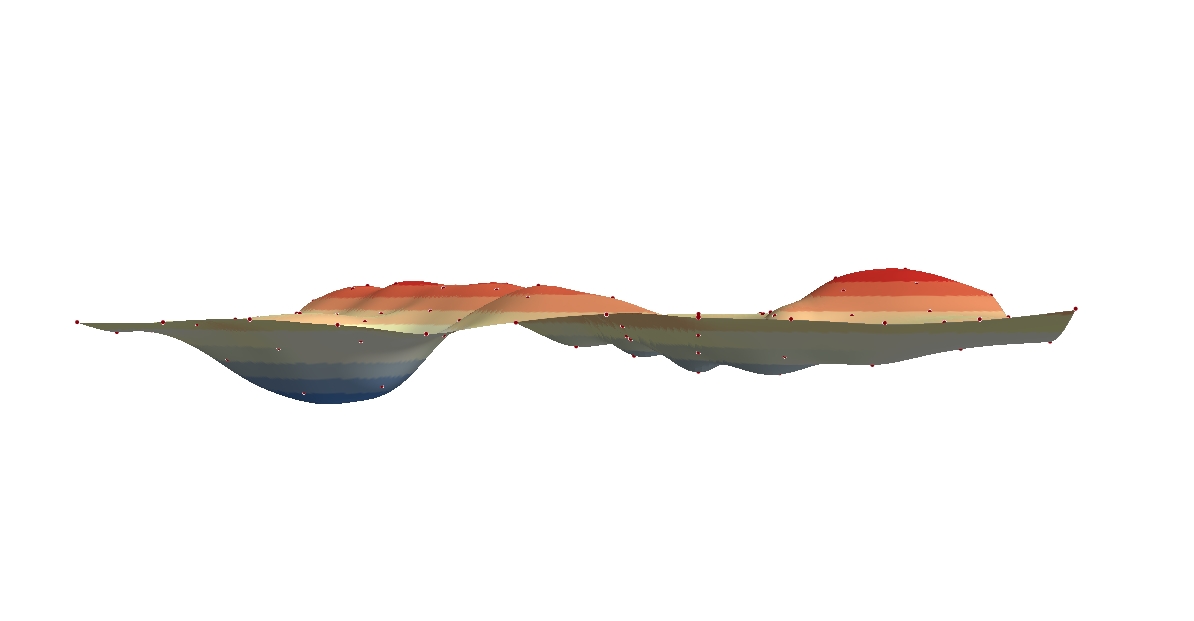
After creating and analyzing the models we decided to resample our area using different sampling protocols in order to create the most spatially accurate model as possible. Because of rain distorting our survey area, it was rebuilt on top of the first, maintaining the same features in the same location (Figure 1).Our group decided to resurvey the entire terrain collecting more XYZ coordinate points at the areas that resulted in accurate modeling such as on slopes and within depressions. Using the new coordinates we reran the interpolation methods to produce a more accurate model.

The goals of this lab were to determine the most efficient surveying techniques to create accurate models. We were to learn about interpolation methods, how to implement them, and the advantages and disadvantages of using each kind of method. We also learned about improving our surveying techniques; balancing collection efforts and data efficiency. This lab taught us very useful survey skills we can implement in a variety of future situations.

Figure 1. Landscape features from left to right: Depression, Ridge, Valley, Hill, Plain

Methods
After we collected the initial survey XYZ data in an Excel spreadsheet and formatted it, the data was imported into ArcGIS and saved in a feature class within a geodatabase created for this lab activity.
Various interpolation methods were performed with the data. ArcGIS Help defines interpolation as predicting values for cells in a raster from a limited number of sample data points. Interpolation is a way to convert individual point values into a continuous raster feature by 'filling in the blanks' between points.  Many different interpolation methods are utilized to achieve different results as required by the surveyor (Figure 2).The rasters and TIN that were created using the methods discussed below were viewed in ArcScene in order to view the models in 3D to better analyze the effectiveness of each.

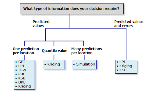Figure 2. Different interpolation methods may be used based on the requirements of the data.

The first method of interpolation used was IDW, or Inverse Distance Weighted technique. This method averages cell values by averaging the values of the points near each cell. The closer a point is to the cell , the more weight it is assigned in the averaging process. Because areas are less accurate the farther away they are from the points, it can cause problems on areas with a steep slope change such as on ridges or valleys.

Figure 3. 3D model of the survey area using the IDW interpolation method. The bumps and pock marks are the result of areas farther away from the coordinate points being weighted less and decreasing the influence of the raster cell.

The second interpolation method that was utilized was the Natural Neighbor method. An advantage of this method is that it doesn't make many assumptions about the data and only takes into consideration the nearest points to determine cell value. Because of this, the Natural Neighbor method is best utilized on projects that require fine detail. This method will not predict trends. This method employs "area stealing" meaning that it uses the nearest coordinate points and weigh them based on their proportionate areas. A disadvantage is that if a cell center falls outside of the convex cell as defined by the input points, those cells will be assigned a value of NoData.

Figure 4. 3D model of the survey area using the Natural Neighbor interpolation method. This method uses "area stealing" based on nearby coordinate points. This results in a smooth surface relative to the IDW method.

The next interpolation method used was Kriging. Kriging creates an estimated surface and utilizes trend to create a raster surface. A disadvantage of Kriging is that it can be processer-intensive if many points are processed. Kriging assumes the presence of a structural component and assumes that local trends vary among locations.

Figure 5. 3D model of the survey using the Kriging interpolation method. Because Kriging takes into account the overall spatial arrangement, it can predict the terrain features using trends.

The fourth interpolation model we tested was Spline. The Spline method used a mathematical function to reduce surface curvature which effectively smoothed the raster to fit perfectly through each coordinate point. Although aesthetically pleasing, some surface features may be ignored if they don't occur directly on the collected coordinate points. Accuracy may be increased by increasing the number of XYZ coordinate points collected.

Figure 6. 3D model of the surveyed terrain using the Spline interpolation method. This method allows for the raster to smoothly fit through each collected coordinate point at the expense of losing the undocumented terrain variation.

The final interpolation method we utilized was TIN, or Triangle Irregular Network. TIN is often used to represent surface morphology digitally. TIN utilizes contiguous triangular facets to create 3D images which is different from the other interpolation methods. TIN preserves the integrity of nodes and edges and is often utilized to accurately model ridges and areas with steeply changing values. A disadvantage is that although it produces an accurate model using the input points, it lacks realism and creates many sharp lines that do not exist in nature.

Figure 7. 3D model of the terrain created by making a TIN. Unlike the rasters, this model uses triangles and maintains the data integrity of all of the input coordinate points.

Initially, our group decided that Spline best represented our surveyed data but we believed that we could improve our surveying techniques and create an even more accurate model. In order to better represent the features in our terrain we altered our coordinate grid and collected some points at a 5cm scale around the features which had a significant terrain change such as the ridge, depression, valley, and hill (Figure 8). The plain feature's data collection was not altered as there was little change in the terrain of that feature.

Figure 8. The collected XYZ coordinate system of the initial survey as compared to the XYZ coordinate system collected in the second survey.

In order to take methods using a 5cm scale at some areas, we marked measurements on masking tape on the frame of the survey box in both 5cm and 10 cm increments (Figure 9).

Figure 9. Marking masking tape on the top of the frame with 5cm and 10cm increments.

In order to make data collection more time efficient and accurate, for the second survey instead of using string we laid a expandable measuring tape across the frame which allowed us to take measurements with another measuring stick without having to move strings for each new point (Figure 10).

Figure 10. A measuring stick was laid across the frame in lieu of string in order to more efficiently and accurately record XYZ coordinate points.

In response to concerns raised during the initial survey, we dug out the outline of the frame so that points with no height features would be flush with 'sea level.' The frame was leveled with a digital level from our smartphones. Because we had to rebuild our feature's surfaces which had been altered from the rain, it was not crucial to match up our initial grid to the subsequent one. In total we collected 218 points as compared to 132 points in the first survey. We hoped that after importing our data into ArcGIS and rerunning the interpolation methods, we would find that our rasters were more representative of the real life terrain. After running the Spline interpolation, we determined that the new model including the more detailed method gave us a more spatially accurate raster (Figure 11).


Figure 11. Model with more XYZ coordinate points than the first survey and a Spline interpolation is a more accurate representation of our terrain.

Discussion
The main issue we faced when tasked with creating a second survey was improving how the data was collected so that the terrain features would be more representative of our physical terrain. We solved this issue by collecting points in between the original coordinate points by measuring 5cm intervals at features that had a significant change in topology that we wanted to account for in our models. The improvements were observed using each of the interpolation methods are shown below.

 

Figure 12, Model of initial survey using the Spline interpolation method. Some terrain features, especially elevation gradients on slopes have been 'averaged out' resulting in an aesthetically pleasing, but slightly spatially inaccurate model.

 

Figure 13. Model of second survey using the Spline interpolation method. By collecting additional points where there were elevation gradients, the features that were smoothed out in the initial survey are now accounted for in the second survey model.

 It is important to realize that our surveys were not perfect replicates of each other due to the need to rebuild the features. However, it is clear that the second method using more XYZ in areas that had gradient changes greatly improved the accuracy of our model.

 Some challenges and sources of error that we ran into were the same as those experienced in the initial survey. Because of the fragile nature of sand based structures, a very delicate hand was needed in order to obtain an accurate measurement while maintaining the integrity of the terrain. Obtaining measurements from surface level was especially hard in the middle of the frame because we could not lean on the frame lest we disturb the leveling nor could we hold ourselves up in the terrain without altering the geography. Abdominal training may have lessened our challenge.

An issue unique to the second survey was the issue of time. The second survey was recorded in the morning, and we finished just in time for me to reach my next class in time. Due to the time crunch we may have been less careful than we would have been otherwise.

A challenge that we solved during the second survey was remembering to dig out where the frame sat in the sand so that areas with no height were at or within a positive sea level value. Light was better in the morning and resulted in more spatially representative photographs.

Conclusion
Although during the second survey we solved many of our issues, I believe that there is still room for improvement, as there is in any project. Packing the sand or keeping it sufficiently wet may help for maintaining terrain integrity and even more XYZ coordinate points may improve our rasters. Although we had to completely resurvey our area, I feel that we improved not only our methods but also the accuracy of our raster. In doing so, we accomplished the main objective of this exercise which was to improve on our survey methods and ability to use interpolation methods to accurately represent a surveyed terrain.

References: ArcGIS Help Online

Evaluation

Lab 1

1. Prior to this activity, how would you rank yourself in knowledge about the topic. (1-No Knowledge at at all, 2-Very Little Knowledge, 3-Some knowledge, 4-A good amount of knowledge, 5-I knew all about this)

I would rate myself as a 3, in that I had some knowledge and somewhat of an idea of how to accomplish the goal.

2.       Following this activity, how would you rate the amount of knowledge you have on the topic (1- I don’t really know enough to talk about the topic, 2- I know enough to explain what I did, 3-I know enough to repeat what I did, 4-I know enough to teach someone else, 5- I am an expert)

I rate myself as a 4; I know enough to teach someone else the concepts. However, there is always room for improvement and I admit that I most likely do not know enough to consider myself an expert.

3.       Did the hands-on approach to this activity add to how much you were able to learn (1-Strongly Disagree, 2-Disagree, 3-No real opinion, 4-Agree, 5-Strongly Agree)

The hands on approach added greatly to what I was able to learn. As a kinesthetic leaner concepts are most easily grasped by physically performing the goal. In lecture the theoretical concept of our goal was almost lost on me.

What types of learning strategies would you recommend to make the activity even better?
I understand that the learning outcome of this lab was to see how we perform with little guidance, but a hard copy of the instructions would have been helpful as I often second guessed my tasks in the beginning.

Exercise 1: Terrain Surface Survey

Introduction
For the first lab assignment in Geospatial Field Methods Geog 336 we were randomly placed in groups of three. I was placed in Group One.

Each group was tasked with creating a unique series of surface features using sand within a four by four foot box. This exercise was to allow us to 'get our hands dirty' and allow us to begin using the geospatial techniques we will utilize often in this course and develop necessary skill sets for further projects and careers.

Methods
Our task was to create a unique landscape within a four by four foot wooden frame. A variety of features was required in order to provide a wide range of data for us to collect and subsequently process into ArcMap for analysis. The features required to be present in our landscape were:
Hill
Valley
Ridge
Depression
Plain

Figure 1 Landscape Features

We were to create these features within our box in our sample plot which was underneath the UWEC campus footbridge near the Haas building on the river floodplain. This area was sandy and reasonably protected from the elements and potential vandals.

We cleared large debris from out site and smoothed the sand slightly. We leveled the frame using a liquid level and additional sand was packed under corners that dipped slightly. Leveling our frame prevented us from having to adjust our data during data processing.

Figure 2 Leveling the frame

Using a shovel and sand from outside of our sample area we created the required features, slightly smoothing them with our hands to allow for less subjective measurements.

Figure 3 Smoothed Features

We applied masking tape to the edges of the frame and marked off 10cm increments with a pen.

Figure 4 10cm Markings

Using two different colors of string held taught on the top edge of the frame we created a 12x11 grid which provided our X and Y values at each crossing point.

Figure 5 Making the grid

Using a meter stick we measured the Z value by noting where the strings reached on the meter stick in centimeters when the bottom-most corner touched the feature point directly below the crossed string. A light hand was needed to prevent the meter stick from going too far into the feature.

Figure 6 Taking Measurements

Zach and I held the string taught at each 10cm mark and took turns reading off the measurements when the other could no longer see it. Peter entered data in Excel using a portable tablet and held the cross string taught with a weight providing resistance on the other end. In total we collected 133 points.

Figure 7 Data Entry

We then measured the height of the frame and determined the factor for 'sea level.' We applied the value to the data and inverted it to determine the actual height of the data points. Unfortunately we forgot to place the frame slightly lower in the sand than our 'flat' areas so we had points with 0 height resulting in a negative value. This is something we will likely change in the subsequent lab.

Discussion 
This lab was beneficial in giving physical tasks to theoretical concepts. As once who learns by doing, this made the concept much more understandable. I was initially unsure of the goals and our means of accomplishing them so I relied on my group members to help get the lab started. Once I began physically working on the tasks the overall goal seemed much more attainable.

Working in teams is usually something I need to work on because I find I am at my most productive when I work by myself. However this lab taught me the importance of allowing your group mates to take charge on a project. Data collection was initially a slow process but once each of us found our place in the task it sped up considerably.

Conclusion
This exercise gave us a useful task to accomplish and required some creative and critical thinking. Once our data is imported into ArcMap and analyzed we will have a better idea of how successful our methods were.

Although some aspects of our methods will be changed in the subsequent lab it gave us a good jumping off point and set the stage for geospatial thinking. Overall this lab was an excellent warmup to what we will accomplish later in the year.